Open main paper 🔗

4  Measuring the dimensions of fairness

Objectives

We describe and quantify fairness disparities along three dimensions: actuarial fairness, solidarity, and causality. These dimensions provide complementary views on how premiums deviate from fairness ideals.

The goal of this chapter is twofold:

• Define operationalizable disparity metrics aligned with each fairness dimension.
• Evaluate and visualize the fairness alignment of benchmark premiums under multiple scenarios.

Disparities are quantified using Wasserstein distances between protected groups. Premiums are then evaluated by their alignment across all dimensions. This informs the selection of premiums with balanced fairness properties.

library(tidyverse)
library(latex2exp)
library(jsonlite)

pregroup_grid_stats <- jsonlite::fromJSON('preds/pregroup_grid_stats.json')
pregroup_pop_stats <- jsonlite::fromJSON('preds/pregroup_pop_stats.json')
preds_sims_stats <- jsonlite::fromJSON('preds/preds_sims_stats.json')

wasserstein_by_group <- function(values, group) {
  # Check inputs
  if (length(values) != length(group)) stop("Length mismatch between values and group.")
  if (length(unique(group)) != 2) stop("Group must be binary.")
  
  # Convert group to factor with two levels
  group <- as.factor(group)
  
  # Split values by group
  values0 <- values[group == levels(group)[1]]
  values1 <- values[group == levels(group)[2]]
  
  # Load transport package for wasserstein1d
  if (!requireNamespace("transport", quietly = TRUE)) {
    install.packages("transport")
  }
  library(transport)
  
  # Compute 1D Wasserstein distance
  return(wasserstein1d(values0, values1))
}

In the case study of the main paper, we briefly discuss how we quantified disparities using the Wasserstein distance. We briefly discuss technical limitations in the measurement of the different disparities regarding the three dimensions of fairness: actuarial fairness, solidarity, and causality.

Related section
The dimensions of fairness are described in Section 3 of the main paper.

4.1 Measuring actuarial fairness disparities

Related section
The measurements associated with the dimensions of fairness are described in Section 4.3 of the main paper.

Actuarial fairness concerns differences in expected loss ratios. Disparity implies cross-subsidies, a violation of actuarial fairness. We compute individual loss ratios as

\[ LR_i = Y_i / \text{premium}_i. \]

We then compare their distributions across protected groups using the Wasserstein distance. Since premiums are strictly positive, individual loss ratios are well-defined.

In cases where claims contain many zeros, aggregated loss ratios over small subpopulations are more stable. We apply this approach in the main paper when appropriate. In our Gaussian case study, individual-level ratios suffice.

4.2 Measuring solidarity disparities

Solidarity demands similar premiums across protected groups. Disparity is measured via the Wasserstein distance between premium distributions: A Wasserstein distance strictly greater than 0 indicates a breach in solidarity.

4.3 Measuring proxy disparities

To assess proxy disparity, we take inspiration from Lindholm et al. (2024) by measuring individual “proxy effects”. Following Côté, Côté, and Charpentier (2024), we measure proxy effects as the difference between a given premium and the aware premium. We then compare their distributions across protected groups. This aligns with the proxy parity criterion of Côté, Côté, and Charpentier (2024). Implicitly, we assume that our estimate of the aware premium is unbiased, otherwise proxy effect assessment may be highly unreliable.

4.4 Disparity measurement per dimension

the_wass_table <- setNames(nm = names(pregroup_pop_stats)) |> lapply(function(the_scenario){
  the_data <- pregroup_pop_stats[[the_scenario]]$valid
    
  setNames(nm = c('mu_B', 'mu_U', 'mu_A', 'mu_H', 'mu_C', 'prem')) |> 
  sapply(function(the_prem){
        the_data$prem_to_eval = the_data[[the_prem]]
    df_to_eval <- the_data |> 
      mutate(to_measure_actuarialfairness = Y/prem_to_eval, # This is the individual loss ratio on which parity per group D is desired
             to_measure_solidarity = prem_to_eval, # This is the premium on which parity per group D is desired
             to_measure_causality = prem_to_eval - mu_A_t # This is the 'proxy effect' on which parity per group D is desired
             ) |> 
      dplyr::select(D, 
                    to_measure_actuarialfairness,
                    to_measure_solidarity,
                    to_measure_causality)
    
    
    lr_disparity <- wasserstein_by_group(values = df_to_eval$to_measure_actuarialfairness,
                                         group = df_to_eval$D)
    prem_disparity <- wasserstein_by_group(values = df_to_eval$to_measure_solidarity,
                                           group = df_to_eval$D)
    proxy_disparity <- wasserstein_by_group(values = df_to_eval$to_measure_causality,
                                            group = df_to_eval$D)
    
    return(
      c('lr_disparity' = round(lr_disparity, 4),
        'prem_disparity' = round(prem_disparity, 3),
        'proxy_disparity' = round(proxy_disparity, 3))
)
  }) |>  t()
})

Scenario 1

library(knitr)
library(kableExtra)
library(DT)

datatable(
  the_wass_table[['Scenario1']] |> 
    as.data.frame() |> 
    mutate(Premium = rownames(the_wass_table[['Scenario1']])) |> 
    dplyr::select(Premium, proxy_disparity, lr_disparity, prem_disparity) |>
  dplyr::rename(
    `Proxy Disparity` = proxy_disparity,
    `LR Disparity` = lr_disparity,
    `Premium Disparity` = prem_disparity
  ),
  
  escape = FALSE,  # enables LaTeX/math rendering
  options = list(
    autoWidth = TRUE,
    dom = 't',      # ONLY table, no filter, no search, no pagination
    columnDefs = list(
      list(className = 'dt-center', targets = 0),
      list(className = 'dt-right', targets = 1:3)
    )
  ),
  rownames = FALSE,
  caption = htmltools::tags$caption(
    style = 'caption-side: top; text-align: left; font-weight: bold;',
    'Scenario 1: Disparity measures as wasserstein distance between D subpopulation distributions. The quantity behind the distribution depends on the dimension measured. '
  )
)

Scenario 2

datatable(
  the_wass_table[['Scenario2']] |> 
    as.data.frame() |> 
    mutate(Premium = rownames(the_wass_table[['Scenario2']])) |> 
    dplyr::select(Premium, proxy_disparity, lr_disparity, prem_disparity) |>
  dplyr::rename(
    `Proxy Disparity` = proxy_disparity,
    `LR Disparity` = lr_disparity,
    `Premium Disparity` = prem_disparity
  ),
  
  escape = FALSE,  # enables LaTeX/math rendering
  options = list(
    autoWidth = TRUE,
    dom = 't',      # ONLY table, no filter, no search, no pagination
    columnDefs = list(
      list(className = 'dt-center', targets = 0),
      list(className = 'dt-right', targets = 1:3)
    )
  ),
  rownames = FALSE,
  caption = htmltools::tags$caption(
    style = 'caption-side: top; text-align: left; font-weight: bold;',
    'Scenario 2: Disparity measures as wasserstein distance between D subpopulation distributions. The quantity behind the distribution depends on the dimension measured. '
  )
)

Scenario 3

datatable(
  the_wass_table[['Scenario3']] |> 
    as.data.frame() |> 
    mutate(Premium = rownames(the_wass_table[['Scenario3']])) |> 
    dplyr::select(Premium, proxy_disparity, lr_disparity, prem_disparity) |>
  dplyr::rename(
    `Proxy Disparity` = proxy_disparity,
    `LR Disparity` = lr_disparity,
    `Premium Disparity` = prem_disparity
  ),
  
  escape = FALSE,  # enables LaTeX/math rendering
  options = list(
    autoWidth = TRUE,
    dom = 't',      # ONLY table, no filter, no search, no pagination
    columnDefs = list(
      list(className = 'dt-center', targets = 0),
      list(className = 'dt-right', targets = 1:3)
    )
  ),
  rownames = FALSE,
  caption = htmltools::tags$caption(
    style = 'caption-side: top; text-align: left; font-weight: bold;',
    'Scenario 3: Disparity measures as wasserstein distance between D subpopulation distributions. The quantity behind the distribution depends on the dimension measured. '
  )
)

4.5 Visualization of alignment with dimensions

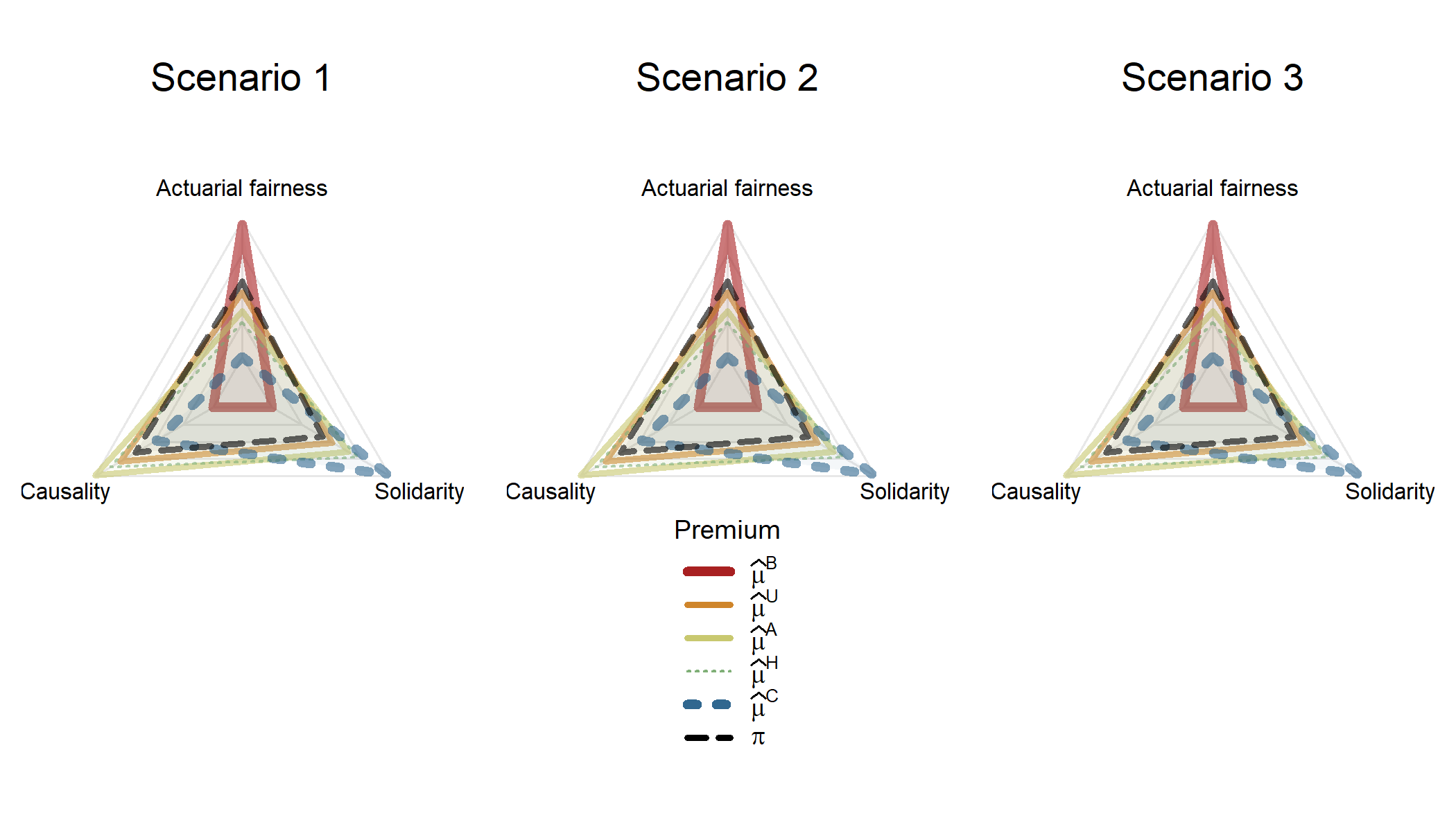
Next, we visualize premium alignment across fairness dimensions. We first standardize the measurements for comparability, then reverse their direction so that higher values indicate better alignment.

the_alignement_table <- setNames(nm = names(the_wass_table)) |> lapply(function(the_scen){
  the_wass_table[[the_scen]] |> 
  data.frame() |> 
  mutate(proxy_disparity = (1 - proxy_disparity/max(proxy_disparity)) |> round(4),
         lr_disparity = (1 - lr_disparity/max(lr_disparity)) |> round(3),
         prem_disparity = (1 - prem_disparity/max(prem_disparity)) |> round(3)) |> 
    mutate(Premium = rownames(the_wass_table[['Scenario3']])) |> 
    dplyr::select(Premium, proxy_disparity, lr_disparity, prem_disparity) |>
  dplyr::rename(
    `Causality` = proxy_disparity,
    `Actuarial fairness` = lr_disparity,
    `Solidarity` = prem_disparity
  )
}) 

if(!file.exists('figs/radar_grid_1x3.png')){
 library(fmsb)
library(colorspace)

# Output
dev_id <-png(paste0("figs/radar_grid_1x3.png"), width = 7, height = 4.0, units = "in", res = 300)

# Then define layout
par(mfrow = c(1, 3), mar = c(0.8, 0.8, 0.0, 0.8), oma = c(1.0, 0.0, 0.0, 0.0))

# Define palette
the_vec <- c(RColorBrewer::brewer.pal(5, 'Spectral'), "black") %>% darken(0.2)
lty_vec <- c("solid", "solid", "solid", "12", "12",  "32")

for (the_scen in names(the_alignement_table)) {
  the_local_table <- the_alignement_table$Scenario1

  data_2 <- the_local_table %>% select(`Actuarial fairness`, Causality, Solidarity)
  data_radar <- rbind(
      c(1, 1, 1),
      c(0, 0, 0),
      data_2
    ) %>% as.data.frame()
  rownames(data_radar) <- c("Max", "Min", the_local_table$Premium)
  
  radarchart(data_radar,
               maxmin = TRUE,
               cglty = 1,
               cglcol = "grey91",
               plty = lty_vec,
               pty = 32,
               pcol = adjust_transparency(the_vec, 0.6),
               plwd = c(4.5, 3, 3, 1.5),
               pfcol = adjust_transparency(the_vec, 0.05),
               vlcex = 1,
               vlabels = c("Actuarial fairness", "Causality", "Solidarity"))
  mtext(paste0('Scenario ', which(the_scen == names(the_alignement_table))), side = 3, line = -3.5, cex = 1.1)
}

# Reset for legend
par(mfrow = c(1, 1), mar = c(0, 0, 0, 0))

## Add a single legend in last panel
legend("bottom",
       title = "Premium",
       legend = latex2exp::TeX(c("$\\widehat{\\mu}^B$","$\\widehat{\\mu}^U$", "$\\widehat{\\mu}^A$",
                                 "$\\widehat{\\mu}^H$", "$\\widehat{\\mu}^C$", "\\pi")),
       bty = "n", col = the_vec,
       text.col = "black",
       cex = 0.75,
       lty = lty_vec, 
       lwd = c(4.5, 3, 3, 1.5),
       xpd = TRUE,
       inset = c(0.2, 0))

dev.off() 
}

Figure 4.1: Alignment of the different benchmark premiums and the given commercial price with the dimensions of fairness.

Scenario 1

datatable(
  the_alignement_table[['Scenario1']],
  
  escape = FALSE,  # enables LaTeX/math rendering
  options = list(
    autoWidth = TRUE,
    dom = 't',      # ONLY table, no filter, no search, no pagination
    columnDefs = list(
      list(className = 'dt-center', targets = 0),
      list(className = 'dt-right', targets = 1:3)
    )
  ),
  rownames = FALSE,
  caption = htmltools::tags$caption(
    style = 'caption-side: top; text-align: left; font-weight: bold;',
    'Scenario 1: Alignment scores across fairness dimensions for each premium. Measures are standardized; a score of 0 denotes the weakest alignment among all premiums for that dimension.'
  )
)

Scenario 2

datatable(
  the_alignement_table[['Scenario2']],
  
  escape = FALSE,  # enables LaTeX/math rendering
  options = list(
    autoWidth = TRUE,
    dom = 't',      # ONLY table, no filter, no search, no pagination
    columnDefs = list(
      list(className = 'dt-center', targets = 0),
      list(className = 'dt-right', targets = 1:3)
    )
  ),
  rownames = FALSE,
  caption = htmltools::tags$caption(
    style = 'caption-side: top; text-align: left; font-weight: bold;',
    'Scenario 2: Alignment scores across fairness dimensions for each premium. Measures are standardized; a score of 0 denotes the weakest alignment among all premiums for that dimension.'
  )
)

Scenario 3

datatable(
  the_alignement_table[['Scenario3']],
  
  escape = FALSE,  # enables LaTeX/math rendering
  options = list(
    autoWidth = TRUE,
    dom = 't',      # ONLY table, no filter, no search, no pagination
    columnDefs = list(
      list(className = 'dt-center', targets = 0),
      list(className = 'dt-right', targets = 1:3)
    )
  ),
  rownames = FALSE,
  caption = htmltools::tags$caption(
    style = 'caption-side: top; text-align: left; font-weight: bold;',
    'Scenario 3: Alignment scores across fairness dimensions for each premium. Measures are standardized; a score of 0 denotes the weakest alignment among all premiums for that dimension.'
  )
)

Côté, Marie-Pier, Olivier Côté, and Arthur Charpentier. 2024. “Selection Bias in Insurance: Why Portfolio-Specific Fairness Fails to Extend Market-Wide.” Available at SSRN: 10.2139/Ssrn.5018749.

Lindholm, M., R. Richman, A. Tsanakas, and M. V. Wüthrich. 2024. “Sensitivity-Based Measures of Discrimination in Insurance Pricing.” Available at SSRN: Ssrn.com/Abstract=4897265.